Lagrangian advection schemes

This is a continuing work of my PhD research, toward a new practical advection scheme constructed in Lagrangian framework which can be applied in the atmospheric general circulation model (AGCM). The advection equation is as following \[ \frac{\partial \rho}{\partial t} + \mathbf{V}\cdot\nabla{\rho} = -\rho\nabla\cdot\mathbf{V} \] The major starting point is to reduce the numerical diffusion error revealed in the Eulerian schemes (including semi-Lagrangian schemes).

Previously, I have constructed two Lagrangian schemes with different discretization fashions, namely TTS-C (Dong and Wang, 2012) and TTS-I (Dong and Wang, 2013). Both of them exhibit lower numerical diffusion as expected.

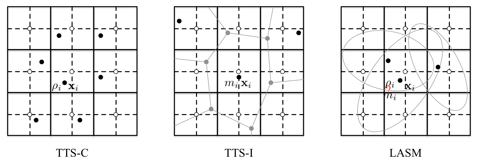
**Fig. 1** The schemas of my three Lagrangian schemes.

In TTS-C, the continuous tracer is discretized into parcel centroids with finite number, which carry tracer density and move around under the influence of the flow. The density is time varying according to the flow divergence, and it is remapped onto the grids of the model (e.g. AGCM) by using the inverse-distance weight (IDW) interpolation. This is the first Lagrangian scheme that I have ever made, so it is simple in concept and shows the good merit of Lagrangian schemes (much lower numerical diffusion). But there are some weak points:

The total mass on the grids is not guaranteed to conserved on the model grids, and it is not possible to define the mass carried by a parcel, since the parcels have no shape and then no definite volume. (Actually, the volume can be defined as in HEL scheme (Kaas et al. 2013).)
There exists aliasing error or spectral blocking, because the parcels have no shape and the remapping procedures involve only distance information, but in deformative flow the parcel shape will no longer keep compact and turn to be long filament espectially in high shear region. (ATTILA (Reithmeier and Sausen 2002) and HEL use mixing among parcels to reduce this error for long time simulation)

To address the above weak points, I wondered how to describe the shape of the parcel. At first, I found out Voronoi diagram that is good at partition space according to given data set. It looks like the cure for my problem and I can let parcel carry mass, but it turned out that the construction of this diagram can not take into account of the flow deformation. Although this path has been blocked, I had an idea that I should use polygon to describe the interface (or shape) of the parcels. So it came out TTS-I with the parcel interface discretized as a polygon in 2D. The details can be found in Dong and Wang (2013) where a complicate curvature guard algorithm has been devised. This algorithm dynamically inserts or removes edges from the polygon to capture the curvature changes in the deformational flow. In the deformation test flow proposed by Nair and Lauritzen (2010), TTS-I showed good performance of preserving discontinuity, filament and tracer correlation. The aliasing error mentioned in Kaas et al. (2013) did not appear! So we can deduce from this observation that the aliasing error is caused by not simulating the shape of parcels. As TTS-C, TTS-I has the vital shortcoming: The polygon is only valid in 2D. When applied to 3D, either the polyhedra or a quasi-2D vertical coordinate should be used. The former will deadly increase the complexity of the scheme and is not practical. The latter will introduce vertical remapping which is not very preferred.

After being in a dilemma for a while, I found the Finite Mass Method (FMM), which uses the linear transformation matrix to describe the shape of parcels. In other words, the parcel can translate, rotate and change size.

Figure 2 is the latest results of LASM, which exhibits the effects of the interparcel mixing. The experiment setup follows the deformation test case (Nair and Lauritzen 2010; Lauritzen et al. 2012) with non-divergent flow. The initial condition is two slotted cylinders that are discontinuous. The left column contains interparcel mixing, whereas the right column does not. So it can be seen that the mixing operation introduces some interparcel mixing, but the degree is highly acceptable.

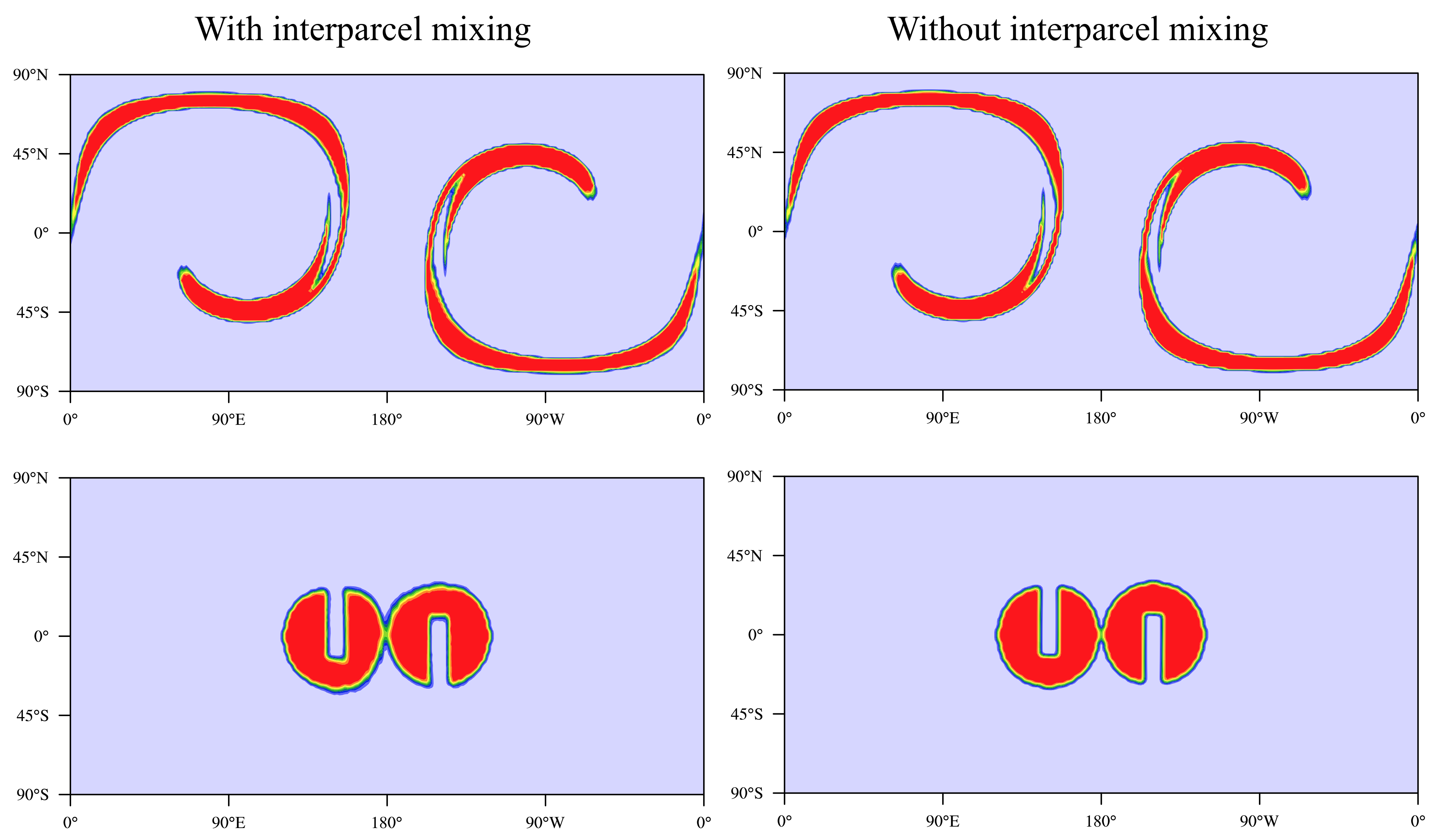
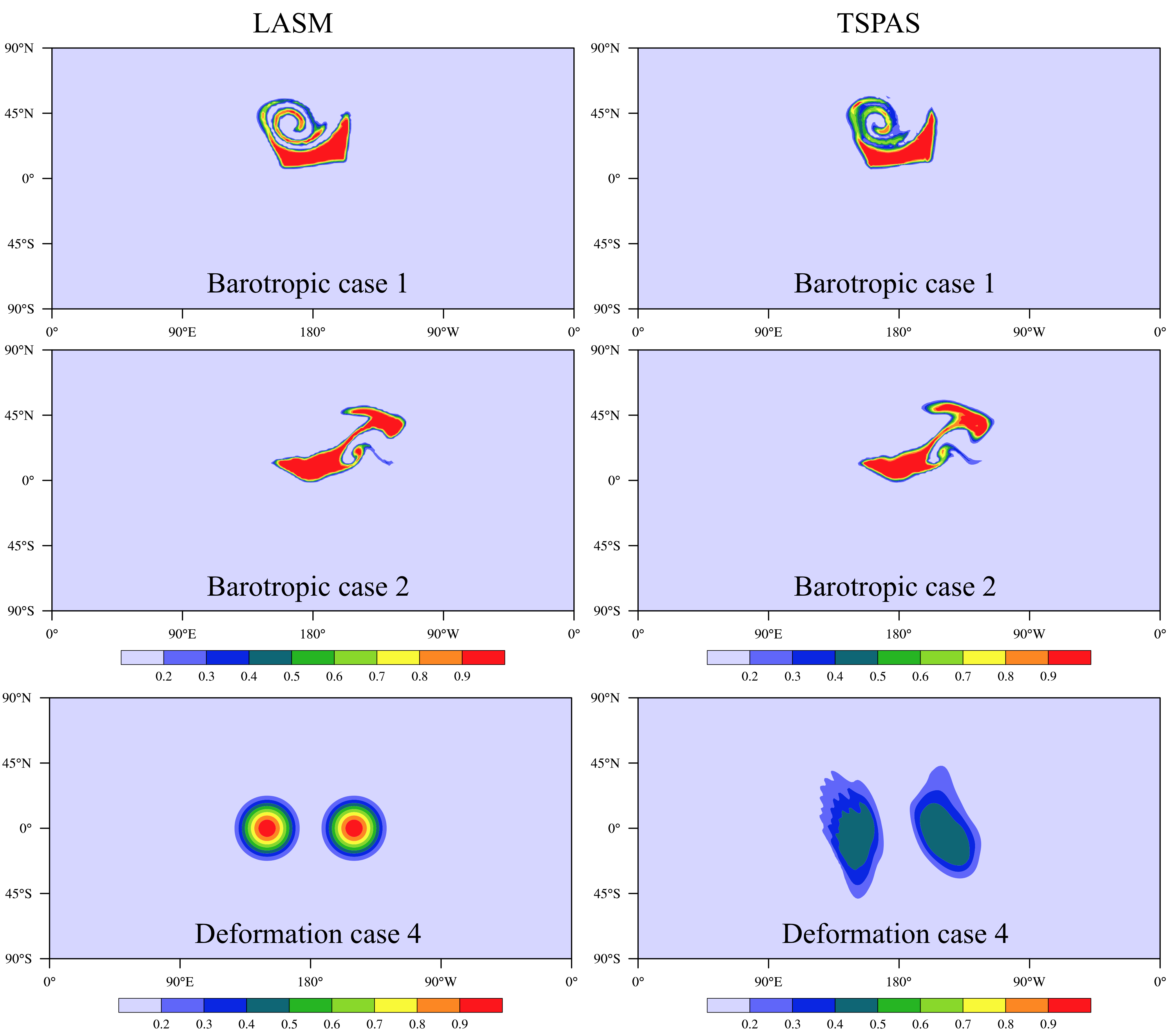
**Fig. 2** The effects of interparcel mixing in LASM shown in deformation test case with the slotted cylinders initial condition. The control parameters are \(\gamma_m\), \(\alpha\), \(\beta_1\) and \(\beta_2\). With smaller \(\gamma_m\), the interparcel mixing will be triggered more easily. \(\beta_2\) controls the degree of lateral mixing, and larger value means less lateral mixing.

Figure 3 is the comparison with TSPAS (Two-step Shape Preserving Scheme, Yu 1994), which belongs the finite difference method. In the ideal deformation case, TSPAS shows unbelievably large errors (e.g numerical diffusion error, shape error), but in the two barotropic cases, TSPAS is more close to LASM, because the flow deformation is not that large as in the deformation case.

**Fig. 3** Comparison between LASM and TSPAS.

The interparcel mixing in LASM is adaptive to the flow so that the mixing is triggered only where the linear deformation approximation of the parcel shape will be violated.

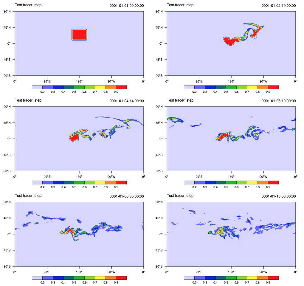
The following is a 10 days barotropic simulation by using a 200hPa wind field and geopotential height from ERA-interim reanalysis data as the initial condition.

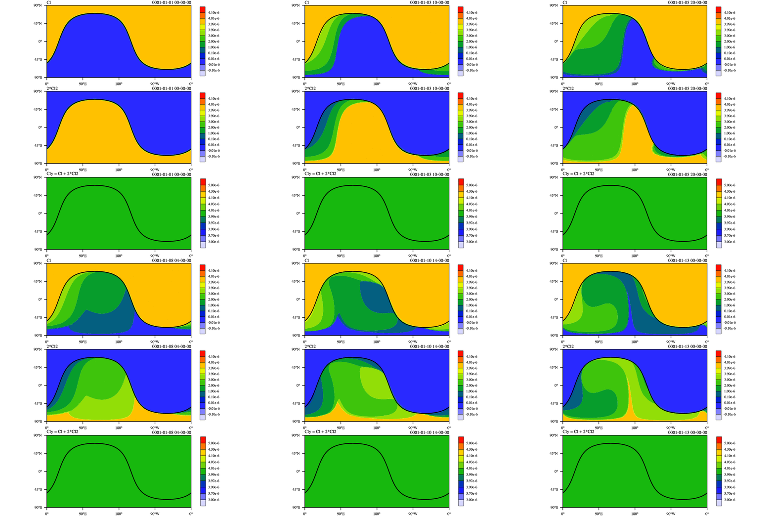
**Fig. 4** 10 days barotropic simulation by LASM (This is an animation, reload if it stops).

I have conducted a newest "terminator toy-chemistry" test case proposed by Lauritzen et al. (2014). This test case examines how well an advection scheme preserves linear correlations. "This chemistry mimics photolysis-driven processes near the solar terminator. As a result, strong gradients in the spatial distribution of the species develop near the edge of the terminator." As you can see, LASM can exactly preserve the linear correlations between two tracers. The results of CAM-FV and CAM-SE can be referred here.

**Fig. 5** The evolution of chemical active \(\text{Cl}\) and \(\text{Cl}_2\) tracers (the upper two figures), and the total chlorine atoms \(\text{Cl}_y = \text{Cl} + 2\text{Cl}_2\) (the lowest one) simulated in LASM.

To be continued ...